I've been keeping track of a bunch of offseason top 25s and such, and I have a fairly good handle on what the preseason conventional wisdom. Let's take a look at a some teams where the T-Rank projections diverge from the conventional wisdom, starting with teams that the T-Rank projections are much higher on than the humans.
Illinois
T-Rank: 15
Humans: 40-ish
The conventional wisdom on the Illini seems to be "intriguing, but not in the top 25." Andy Katz is more bullish, putting them at 19th in his latest "Power 36," but T-Rank's No. 15 is well above the median opinion.
I think this is driven by a few things.
First, Illinois returns some sophomores who were promising as freshmen, including a borderline one-and-done in Ayo Dosunmu. The model expects improvements out of those kinds of guys, and big improvement out of Ayo.
Second, the model still likes Brad Underwood based on his well-above-par performances at Stephen F. Austin and Oklahoma St. Humans are not so sold on Underwood, and there's quite a bit of skepticism that his particular system, especially on defense, can work at the high major level.
Third, T-Rank thought Illinois was better last year than most people (and other systems like Kenpom) did. This can have an effect on the defensive projection, which uses prior performance as a baseline.
My take. This is definitely a best-case scenario projection for Illinois, and I'd be much more comfortable with them in the lower 20s even as an optimistic case. There are things to like about this team, and plausible bases to expect a significant leap, but still many question marks and things that could easily go wrong. So I'd go with the conventional wisdom on this one.
Missouri
T-Rank: 13
Humans: Bubble team at best
This is definitely the biggest outlier in the projected top 40. As far as I can tell, no human is expecting anything out of this Missouri squad. Only mention I've seen is they come up 64th in Kevin Sweeney's top 100.
The case against Missouri is straightforward. They were mediocre last year (68th in Kenpom), they lose their most impactful player (Jordan Geist), and they don't have a highly touted freshman class coming in.
As with Illinois, my model's baseline for Missouri is a bit higher on Missouri's past performance; T-Rank had them 54th last year, which is higher than anyone else had them. Most importantly, it had them No. 36 in adjusted defensive efficiency, and 37th the year before. Add in the fact that Cuonzo Martin has a history as a solid defensive coach and that Missouri returns a solid core of defensive players, and I don't have a big problem with the projection for Missouri to be the 25th best defensive team next year.
Where things get a bit wacky is the projection for Missouri to have the No. 15 offense. The offensive projection is mainly player-based, and the short story here is that the model just likes these players together. Mark Smith and Jeremiah Tilmon are juniors who were highly rated recruits, which bodes well for their chance to continue improving into key, reliable offensive players. Torrence Watson, Xavier Pinson, and Javon Pickett are returning sophomores who got good experience as freshmen. And Dru Smith is a transfer from Evansville (a decent mid-major) who was very efficient there as a sophomore.
My take. As with Illinois, I'd find this more defensible if they were in the low 20s or so, because I can sort of get where the model is coming from in liking these players. But I'm not placing or taking any bets premised on Missouri as a top-20 team that contends for an SEC title.
Penn St.
T-Rank: 19
Humans: 50-ish
Penn St. has been a pretty decent team, efficiency-wise, the last two years. Two years ago, they won the NIT and finished 19th in the Kenpom ratings. Last year they finished 43rd at Kenpom. (T-Rank had them 16th and 32nd the past two years, so even a little higher.)
But the perception of this team does not quite track those efficiency numbers. They were never seriously in consideration for an at-large berth either year, mainly because of their 6-20 record in "Quadrant 1" games. Starting 0-10 in the Big Ten last year also didn't help. There's a feeling, I think, that PSU's efficiency numbers are goosed by mopping up against lesser competition, and that Pat Chambers just doesn't have the chops to really compete at the top of the Big Ten.
So the popular opinion on Penn State, I think, is they they were mediocre with a low ceiling last year, and they'll be similar this year after losing Josh Reeves and the unexpected transfer of Rasir Bolton. Yes, they return Lamar Stevens, who puts up big counting stats but does so inefficiently. So it's easy to imagine this being the classic PSU team that features one guy who takes all the shots and that plays pretty hard enough on defense.
My take. 19 is too high, but it's worth noting that Penn State was 24th in a sneak peak of Kenpom's preseason ratings, so at least T-Rank isn't out on an island with this one. Maybe this will be the year that PSU's results more closely align with their efficiency numbers.
Notre Dame
T-Rank: 22
Humans: 50-ish
I've seen surprisingly little love for Notre Dame this offseason. The Irish struggled last year, especially after Rex Pflueger got hurt after ten games. Three top-100 freshmen (Nate Laszewski, Dane Goodwin, and Prentice Hubb) were forced into more action than they were probably ready for.
But Pflueger is back for a fifth year, along with fellow seniors TJ Gibbs and John Mooney. And those three top-100 freshmen are back, poised to make the sophomore leap.
My take. Notre Dame has been a bit snakebitten since Bonzie Colson's injury in 2018. If they stay healthy this year, I think there's a good chance that they are a top 25 team again.
Showing posts with label T-Rank. Show all posts
Showing posts with label T-Rank. Show all posts
Sunday, September 1, 2019

Monday, September 17, 2018
T-Rank Methodology Update
For the first time since 2014, I'm making significant changes to the T-Rank ratings. The output will be the same: adjusted offensive and defensive efficiencies, used to create the "Barthag" pythagorean expectancy. But I've changed how I create the adjusted efficiencies.
Specifically, I'm going to incorporate the "GameScript +/-" stat that I derive from the play-by-play (where available), and I'm going to alter the GameScript stat so that it disregards anything that happens during "garbage time." The resulting ratings will therefore more reflect how well teams actually perform when the outcome is still in question.
In my backtesting, the new ratings perform slightly better than the old ones. But frankly I just thought it would be cool to incorporate this sort of unique data I track, so I went ahead and did it. All the ratings on the site have been updated, back to 2008 (though I don't have any GameScript data for 2008 or 2009, so there are no substantive changes for those years).
In my backtesting, the new ratings perform slightly better than the old ones. But frankly I just thought it would be cool to incorporate this sort of unique data I track, so I went ahead and did it. All the ratings on the site have been updated, back to 2008 (though I don't have any GameScript data for 2008 or 2009, so there are no substantive changes for those years).
Details:
Wonky note: the new ratings have a narrower "spread" in the adjusted efficiencies, so I've upped the "exponent" used to calculate the Barthag from 10.25 to 11.5. I'm sure this will cause some bugs on the site, so please let me know if you notice any weirdness.
For the past two seasons I have produced separate ratings, the "Implied T-Rank," using the GameScript stat. What I do is use the GameScript stat—which represents a team's average lead or deficit during a game—to infer a final score, and then use this derived final score instead of the actual final score to create the ratings.
To explain how I get this derived final score, I'll use Wisconsin's home game against Michigan last year, which is a good example of a game where the actual final score (83-72, Michigan) gives a different picture than the GameScript (Michigan +14.5 when its lead became safe, which is equivalent to about a 29-point win):
1) Calculate the GameScript using play-by-play data. Going forward I will use the GameScript at the moment the winning team's lead becomes "safe" (using Bill James's famous formula), unless there is a miraculous comeback. Thus, the GameScript will not reflect any scoring during "garbage time," whether it's running up the score or the scrubs coming in to allow the final number to be more respectable. As it reflects a team's average lead/deficit over the entire game, GameScript was already resistant to late-game shenanigans (it can change only so much in the last few minutes, no matter what happens), but this will make it even more so.
2) To derive a score, add up both teams' actual scores, divide that by two, then add or subtract the GameScript. In the case of the Michigan at Wisconsin game, there were 155 points scored, so Michigan's derived score would be 77.5 + 14.5 = 92 and Wisconsin's derived score would be 77.5 - 14.5 = 63. Derived score is Michigan, 92-63. That's the 29-point margin.
The new T-Rank will use both the actual score and this GameScript-derived score (where available) from each game to calculate adjusted offensive and defensive efficiencies, and then everything else will be the same.
One potentially controversial aspect of this method is that a team can win the game but have a negative GameScript, and therefore have its "derived" score be a loss. To somewhat mitigate this, I divide the GameScript in half in those situations.
Wonky note: the new ratings have a narrower "spread" in the adjusted efficiencies, so I've upped the "exponent" used to calculate the Barthag from 10.25 to 11.5. I'm sure this will cause some bugs on the site, so please let me know if you notice any weirdness.
Sunday, January 14, 2018
Teamcast tip: note the Projected T-Rank variable
One of the newer features over at the T-Rank site is a tool I call "Teamcast," which lets you select the results of a team's games and shows how those results would affect the T-Ranketology forecast.
I'm not gonna lie, I think this is a pretty awesome tool and I play around with it a lot. But of course there are some pretty important caveats to keep in mind:
1) The underlying T-Ranketology algorithm is not a crystal ball. Although it performed really well last year, last year was a pretty predictable year. In retroactive investigations, T-Ranketology does "pretty good" for prior years too. But overall it's safe to say that you should consider any T-Ranketology forecast to have at least a +/- one-seed margin of error.
2) There's reason to believe that this year will be much less predictable than prior years, because the Committee will be considering new and different information (most importantly, the new quality win quadrants). We can only presume how the Committee will use the new information. My guess is that they will use it to make some ... unpredictable ... choices.
That said, the Teamcast is still a fun tool, and at the very least it should be pretty good for looking at relative changes. If it's predicting your team to be an 8-seed, and picking it to win a game moves them up 4 spots to a 7-seed, it's reasonable to say the win was worth about one seed-line—even if it was actually from a 10 to a 9, or a 6 to a 5.
One important thing that gets overlooked, I think, by people playing around with the tool is that the current T-Rank rating plays a role. First, it is obviously how predictions for future games are calculated. Second, it is an independent variable in the T-Ranketology algorithm, and a not insignificant one. (Not because I think the committee is using it, but as a good-enough proxy for other ratings like Kenpom that the committee is using.)
So particularly if you are exploring an extreme scenario, like say, "What would happen if my team won the rest of its games?" you might get a weird result if you do not change the projected T-Rank as well. Because in the scenario where your team wins out, its T-Rank is probably going to improve a lot.
Fortunately, the Teamcast tool lets you change the projected T-Rank (right at the top of the page), which fixes this problem. In fact, simply changing the projected T-Rank and doing nothing else is a pretty good way to use Teamcast earlier in the season. E.g., keep upping the projected T-Rank until your team gets in the field, and that shows how well your team will have to play the rest of the way to likely make the tournament.
ADDED: One way I've attempted to automate this is the "DynamaRank" feature. Basically, this estimates changes to power ratings (including NET) based on the changed results. So this box should be checked for any extreme scenarios where a team loses or wins a lot more games than expected.
If you get any funky results with the Teamcast, or have ideas for improvement, please let me know.
I'm not gonna lie, I think this is a pretty awesome tool and I play around with it a lot. But of course there are some pretty important caveats to keep in mind:
1) The underlying T-Ranketology algorithm is not a crystal ball. Although it performed really well last year, last year was a pretty predictable year. In retroactive investigations, T-Ranketology does "pretty good" for prior years too. But overall it's safe to say that you should consider any T-Ranketology forecast to have at least a +/- one-seed margin of error.
2) There's reason to believe that this year will be much less predictable than prior years, because the Committee will be considering new and different information (most importantly, the new quality win quadrants). We can only presume how the Committee will use the new information. My guess is that they will use it to make some ... unpredictable ... choices.
That said, the Teamcast is still a fun tool, and at the very least it should be pretty good for looking at relative changes. If it's predicting your team to be an 8-seed, and picking it to win a game moves them up 4 spots to a 7-seed, it's reasonable to say the win was worth about one seed-line—even if it was actually from a 10 to a 9, or a 6 to a 5.
One important thing that gets overlooked, I think, by people playing around with the tool is that the current T-Rank rating plays a role. First, it is obviously how predictions for future games are calculated. Second, it is an independent variable in the T-Ranketology algorithm, and a not insignificant one. (Not because I think the committee is using it, but as a good-enough proxy for other ratings like Kenpom that the committee is using.)
So particularly if you are exploring an extreme scenario, like say, "What would happen if my team won the rest of its games?" you might get a weird result if you do not change the projected T-Rank as well. Because in the scenario where your team wins out, its T-Rank is probably going to improve a lot.
Fortunately, the Teamcast tool lets you change the projected T-Rank (right at the top of the page), which fixes this problem. In fact, simply changing the projected T-Rank and doing nothing else is a pretty good way to use Teamcast earlier in the season. E.g., keep upping the projected T-Rank until your team gets in the field, and that shows how well your team will have to play the rest of the way to likely make the tournament.
ADDED: One way I've attempted to automate this is the "DynamaRank" feature. Basically, this estimates changes to power ratings (including NET) based on the changed results. So this box should be checked for any extreme scenarios where a team loses or wins a lot more games than expected.
If you get any funky results with the Teamcast, or have ideas for improvement, please let me know.
Saturday, October 21, 2017
T-Rank: New Stuff for 2017-18 ICYMI MEGAPOST
I've added a bunch of stuff to the T-Rank site this offseason (or at least since the start of last season) and thought it might be a good idea to inventory & explain it somewhere. Somewhere like here.
First, a little back-patting. Three different aspects of the T-Rank site were validated as pretty useful last year: the ratings system itself, the "T-Ranketology" tourney predicting algorithm, and the preseason projections.
The rating system performed well. In terms of predicting games, it was the best full-season predictor, at least according to this analysis. At the very least, T-Rank is in the same league with Kenpom (no surprise, since I copied Kenpom liberally) and Sagarin. This means the adjusted efficiencies that drive the ratings are likely sound as well, and all the fun stuff that I use those adjusted efficiencies to power has at least some relation to reality.
The T-Ranketology algorithm did a great job last year, finishing near the very top of the Bracket Matrix competition. Of course, this was probably lucky, and last year was a bit of a strange year in that most people were able to correctly pick the field. But again, the main takeaway is that T-Ranketology is "good enough" to use for other fun stuff, such as the new Teamcast and Tourneycast features, and feel confident that the results are at least worth taking seriously.
Finally, last year's preseason projections turned out the be the best 1 to 351 projections, at least according to Dan Hanner's analysis. This is somewhat of a bittersweet victory because—as I've explained in an update to this old post—I have actually totally revamped the preseason projections for this year. But I'm confident that the new system is even better, and I'm also quite certain that last year's "victory" was mostly luck. Still, coming out ahead of Hanner and Kenpom by any metric at least shows that the ideas behind the system aren't garbage.
So putting these three facts together, I think it's safe to say that T-Rank's underlying algorithms and ideas are reasonably sound, which makes the tools on the site even more fun to play around with. Speaking of those tools:
This is probably the coolest thing I've added: a tool to play around a team's schedule (picking wins and losses, adding dropping games) to see how it affects their tourney chances and seed, based on the T-Ranketology algorithm.

The last two columns there show how much of an effect a win or loss would have on a team's T-Ranketology score (in isolation from all other games). Teamcast is also retroactive back to 2008, so you can go back and look what would might have happened if a certain game had come out differently.
I'm excited for Teamcast this year to play out various bubble scenarios—especially given the likelihood that the Badgers will be on the bubble.
Daycast is similar to Teamcast, except that instead of playing around with a team's schedule, you play around with the games on a given day to see how it affects the tourney. As part of this, I've developed a new thrill quotient, the "Torvik Tourney Thrill Quotient" or "T3Q" which ranks games in their anticipated effect on the tourney. Basically, games between potential bubble teams reign supreme.

For TourneyCast, I run 10,000 simulations of the season (including simulations of every conference tournament), run the results of each sim through the T-Ranketology algorithm to get a projected field of 68, and then simulate the NCAA tournament. The output is odds for every team to get to the tournament (whether through an autobid or at-large) and then odds for advancing to various stages of the tourney.


Not sure exactly when I did this, but the site is completely backfilled with team and player stats all the way back to 2008. This includes advanced stats boxscores, which certain other sites don't have back past 2011.
The only exception to this is play by play based stats (win probability, game score). I have a complete set of PBP for last year (2017) and 95% coverage for 2015 and 2016. I will probably add more backfill on that in the coming months, but my impression is that available PBP peters out around 2011 anyhow.
This also includes conference-only advanced stats, and all the other various ways I've got to split the player stats, back to 2008. Notable other sites have conference-only advanced stats back to just the 2014 season.
As I just mentioned, I've added new ways to split player stats in the pretty awesome Player Finder tool. Now you can filter out the stats so you look at performance against only top 50 (adjusted for venue) opponents. You can even filter by date, to see who the stars of November were. I've also added a "max height" filter so you can see who the best short rebounder is, for example.
Part of the backfill is that I have advanced player stats back to 2008, including game logs. In addition, one of my major projects this summer was to create a linked database of player histories, so that when you click on a player's name, all his seasons come up. You cannot imagine what a supreme pain in the ass this was. The things I had to learn, I shit you not, were things like natural language processing. Woo boy. But at this point the player histories are about 99% linked. If you see any any discrepancies, please let me know.
I just learned how to make some awesome interactive charts and graphs, replacing the old jpeg-based graphs it took me a week to learn how to make. Pretty proud of myself. This new skill is on display in three areas:
Old:


Every team page has strength of schedule stats, and there's also a comprehensive page for strength of schedule. These are broken down by overall SOS and non-conference SOS, and also broken down by the SOS so far, and projected SOS for the entire season. (Conference SOS calculations are on the conference pages.)
Might as well say a word about my SOS metrics, since they're a bit unusual. The "basic" metric is just the average of the team's opponents' pythagorean expectancy (adjusted for the location of the game).
The "elite" metric is different, and better. This is the percentage of games an "elite" team (approx .9000 Barthag) would be expected lose against a given schedule. This is better because it reflects how little difference there is between playing mediocre and bad teams at home, and really rewards playing games that a good team could realistically lose.
To see what this is better, imagine three potential opponents: one good team (Barthag of .9000), one mediocre team (.5000), and one terrible team (.1000). Under the basic method, playing two mediocre teams is the same as playing a good team and terrible team because (.5 + .5) / 2 = (.9 + .1) / 2. But this really isn't right for most teams that we care about, because an elite team's chances of losing to the mediocre team (at home, at least) aren't really that different than its chances of losing to the terrible team, while its chances of beating the elite team are quite a bit different: (.05 + .01) / 2 < (.50 + .01) / 2.
A concise way to look at team and coach performance back to 2008.
I blogged about the underlying analysis here: I run simulations to see how differently teams would perform against a true round robin schedule (both winning percentage and chance of winning the conference) and log the results.
Here's one I forgot about: a page showing the projected RPIs of every team based on their current T-Rank rating. This page also shows projected records in each of the selection committees newly delineated "quality win" buckets. If you hover over those records, you can see which teams are in each bucket:

First, a little back-patting. Three different aspects of the T-Rank site were validated as pretty useful last year: the ratings system itself, the "T-Ranketology" tourney predicting algorithm, and the preseason projections.
The rating system performed well. In terms of predicting games, it was the best full-season predictor, at least according to this analysis. At the very least, T-Rank is in the same league with Kenpom (no surprise, since I copied Kenpom liberally) and Sagarin. This means the adjusted efficiencies that drive the ratings are likely sound as well, and all the fun stuff that I use those adjusted efficiencies to power has at least some relation to reality.
The T-Ranketology algorithm did a great job last year, finishing near the very top of the Bracket Matrix competition. Of course, this was probably lucky, and last year was a bit of a strange year in that most people were able to correctly pick the field. But again, the main takeaway is that T-Ranketology is "good enough" to use for other fun stuff, such as the new Teamcast and Tourneycast features, and feel confident that the results are at least worth taking seriously.
Finally, last year's preseason projections turned out the be the best 1 to 351 projections, at least according to Dan Hanner's analysis. This is somewhat of a bittersweet victory because—as I've explained in an update to this old post—I have actually totally revamped the preseason projections for this year. But I'm confident that the new system is even better, and I'm also quite certain that last year's "victory" was mostly luck. Still, coming out ahead of Hanner and Kenpom by any metric at least shows that the ideas behind the system aren't garbage.
So putting these three facts together, I think it's safe to say that T-Rank's underlying algorithms and ideas are reasonably sound, which makes the tools on the site even more fun to play around with. Speaking of those tools:
Teamcast
This is probably the coolest thing I've added: a tool to play around a team's schedule (picking wins and losses, adding dropping games) to see how it affects their tourney chances and seed, based on the T-Ranketology algorithm.
The last two columns there show how much of an effect a win or loss would have on a team's T-Ranketology score (in isolation from all other games). Teamcast is also retroactive back to 2008, so you can go back and look what would might have happened if a certain game had come out differently.
I'm excited for Teamcast this year to play out various bubble scenarios—especially given the likelihood that the Badgers will be on the bubble.
Daycast
Daycast is similar to Teamcast, except that instead of playing around with a team's schedule, you play around with the games on a given day to see how it affects the tourney. As part of this, I've developed a new thrill quotient, the "Torvik Tourney Thrill Quotient" or "T3Q" which ranks games in their anticipated effect on the tourney. Basically, games between potential bubble teams reign supreme.
TourneyCast™
For TourneyCast, I run 10,000 simulations of the season (including simulations of every conference tournament), run the results of each sim through the T-Ranketology algorithm to get a projected field of 68, and then simulate the NCAA tournament. The output is odds for every team to get to the tournament (whether through an autobid or at-large) and then odds for advancing to various stages of the tourney.
ADDED: one cool feature of the TourneyCast is that if you filter by conference you get the projected number of bids, at-large chances (interesting for mid-majors), final four chances, and championship chances.
Backfill to 2008
Not sure exactly when I did this, but the site is completely backfilled with team and player stats all the way back to 2008. This includes advanced stats boxscores, which certain other sites don't have back past 2011.
The only exception to this is play by play based stats (win probability, game score). I have a complete set of PBP for last year (2017) and 95% coverage for 2015 and 2016. I will probably add more backfill on that in the coming months, but my impression is that available PBP peters out around 2011 anyhow.
This also includes conference-only advanced stats, and all the other various ways I've got to split the player stats, back to 2008. Notable other sites have conference-only advanced stats back to just the 2014 season.
More Player Stats Splits and Filters
As I just mentioned, I've added new ways to split player stats in the pretty awesome Player Finder tool. Now you can filter out the stats so you look at performance against only top 50 (adjusted for venue) opponents. You can even filter by date, to see who the stars of November were. I've also added a "max height" filter so you can see who the best short rebounder is, for example.
Player Histories and Game Logs
Part of the backfill is that I have advanced player stats back to 2008, including game logs. In addition, one of my major projects this summer was to create a linked database of player histories, so that when you click on a player's name, all his seasons come up. You cannot imagine what a supreme pain in the ass this was. The things I had to learn, I shit you not, were things like natural language processing. Woo boy. But at this point the player histories are about 99% linked. If you see any any discrepancies, please let me know.
Charts and graphs! Charts and graphs!
I just learned how to make some awesome interactive charts and graphs, replacing the old jpeg-based graphs it took me a week to learn how to make. Pretty proud of myself. This new skill is on display in three areas:
Win probability charts
I blogged about my fun foray into created a win probability model here. I've now learned how to make the result more useful and interactive.
Old:

New:
Also: Win probability calculator.
Team Trends Charts
Previously, I had team trends charts for just offensive and defensive efficiency, and they were pictures like the old win prob chart. Now I've got em for most team stats, and they are interactive and fabulous. Note: these charts are also available at the bottom of the "Team Results" page.Player Stats Trends
Not to be done, the player stats department demanded access to the charts and graphs technology.Strength of Schedule Stats & Page
Every team page has strength of schedule stats, and there's also a comprehensive page for strength of schedule. These are broken down by overall SOS and non-conference SOS, and also broken down by the SOS so far, and projected SOS for the entire season. (Conference SOS calculations are on the conference pages.)
Might as well say a word about my SOS metrics, since they're a bit unusual. The "basic" metric is just the average of the team's opponents' pythagorean expectancy (adjusted for the location of the game).
The "elite" metric is different, and better. This is the percentage of games an "elite" team (approx .9000 Barthag) would be expected lose against a given schedule. This is better because it reflects how little difference there is between playing mediocre and bad teams at home, and really rewards playing games that a good team could realistically lose.
To see what this is better, imagine three potential opponents: one good team (Barthag of .9000), one mediocre team (.5000), and one terrible team (.1000). Under the basic method, playing two mediocre teams is the same as playing a good team and terrible team because (.5 + .5) / 2 = (.9 + .1) / 2. But this really isn't right for most teams that we care about, because an elite team's chances of losing to the mediocre team (at home, at least) aren't really that different than its chances of losing to the terrible team, while its chances of beating the elite team are quite a bit different: (.05 + .01) / 2 < (.50 + .01) / 2.
Coach History and Team History pages.
A concise way to look at team and coach performance back to 2008.
Advanced Analysis of Unbalanced Conf. Schedules
I blogged about the underlying analysis here: I run simulations to see how differently teams would perform against a true round robin schedule (both winning percentage and chance of winning the conference) and log the results.
RPI Forecast
Here's one I forgot about: a page showing the projected RPIs of every team based on their current T-Rank rating. This page also shows projected records in each of the selection committees newly delineated "quality win" buckets. If you hover over those records, you can see which teams are in each bucket:
Saturday, July 22, 2017
How I built a (crappy) basketball win probability model
The Internet is amazing. Given that I'm a philosophy major / lawyer, I really have no knowledge or skills whatsoever. But I've been able to put together the T-Rank website by just asking the Internet how to do it. Every time I run into a problem, I just ask google how to solve it. Usually this leads me to more or less step-by-step instructions on how to solve the problem, or at least gives me enough information to figure it out.
There has been one big exception to this: for a while I have wanted to see if could use play-by-play data to build a "win probability model." Not a good win probability model, just a sort of functioning win probability model. Not for any good reason, just because. But my google searches came up empty. Not only were there no step-by-step guides, there weren't even any general instructions to set me down the right path. I was lost. Harumphf.
Nevertheless, I persisted. Although I have no independent "knowledge" or "skills" I do have an epidemiologist wife who does, so one day while we were waiting in the office of a pediatric specialist (don't worry, it was a nothingburger) I ran the problem by her. I had learned just enough by then to explain the problem somewhat coherently, and she was able to set me down the right path.
Now I thought I would fill the void and put a step-by-step guide on to the Internet, mainly so future lawyers can build their own deeply flawed basketball win probability models. Also, if anybody who knows something about this stuff wants to help me improve this, just because, that would be terrific.
Step 1: Get the data.
Okay, I'm not going to walk you through this part, but obviously if you're going to use play-by-play data to make a win probability model, you need play-by-play data. Luckily, there is play-by-play data on various websites, and using google and a little pluck you can figure out how to get it. I started acquiring this data last season to calculate the "game script" average lead/deficit stat. Unfortunately, to get a complete set of data I had to use three different sources, which leads to some problems later on... (This is not just a step-by-step guide, it's also kind of a suspense novel.)
Step 2: Make the model.
Now the easy part: make your model. Done! Thanks for reading my guide.
Now you feel my pain, folks.
Step 2, actually: Figure out what kind of model you need.
This is the point when you have to figure how what you're going to do with the data. What I eventually figured out is that I was going to run use the data to run a "logistic regression." As I understand it (and really, I don't understand it), you can use this statistical method to take various variables (like score, time left, strength of teams) to predict the likelihood of another variable (win or loss, 1 to 0).
It's one thing to know that you need to a "run a logistic regression" and quite another to actually do it. As we'll see below.
Step 3: Get PBP data ("training data") into usable form.
Here's what I did: I went through (most) of the play-by-play data I have for the past two seasons, and for every second of those games I recorded the following data:
1. Seconds remaining
2. Score difference (team 2 score minus team 1 score)
3. team 2 initial expected win percentage (based on T-Rank)
4. who won (team 2 win = 1, team 2 loss = 0)
I actually recorded some more data, but this is what I ended up using for the current model.
One thing you might notice that's missing: who has the ball. This is a big flaw in my model, and I'll discuss it more below. (Suspense!) But for the moment I'll just say that although this is a big flaw, I don't think it really makes much difference until the last two minutes.
Another thing that's missing is home court. This is another thing I left out mainly because it was kind of a pain to figure out based on the PBP data. But, also, home-court advantage is already built in to the third variable (expected win%), so there could be kind of a double-counting problem if I included it separately. I dunno, gimme a break.
Step 4: Run the logistic regression for each second
This might not be the best way, but what I did is run a logistic regression for each of the "seconds remaining" variables (2399, 2388, ... 2, 1, 0), with score difference and initial win percentage as the variables for predicting win/loss (I don't know the proper nomenclature for discussing regression, so bear with me).
Originally I ran a single regression with time remaining as another one of the variables, but the results were unsatisfactory, particularly at the margins. For example, it was obviously wrong very early in the game — I think because linearity was being imposed, but not sure. Anyhow, running it for every second worked out pretty nicely.
As I mentioned above, saying "run a logistic regression" and actually doing it are different things, so here's how I did it: I used Python, a programming language, which has a module for doing this called LogisticRegression. Here's a link to the code.
Step 5: Test it, see if it passes the smell test
The result of this model is that you can plug in "seconds remaining" (to get the right model), score (in the form of score differential), and initial win percentage expected to get an expected win probability.
For example, here's the result using Minnesota versus Middle Tennessee in last year's NCAA tourney:


There has been one big exception to this: for a while I have wanted to see if could use play-by-play data to build a "win probability model." Not a good win probability model, just a sort of functioning win probability model. Not for any good reason, just because. But my google searches came up empty. Not only were there no step-by-step guides, there weren't even any general instructions to set me down the right path. I was lost. Harumphf.
Nevertheless, I persisted. Although I have no independent "knowledge" or "skills" I do have an epidemiologist wife who does, so one day while we were waiting in the office of a pediatric specialist (don't worry, it was a nothingburger) I ran the problem by her. I had learned just enough by then to explain the problem somewhat coherently, and she was able to set me down the right path.
Now I thought I would fill the void and put a step-by-step guide on to the Internet, mainly so future lawyers can build their own deeply flawed basketball win probability models. Also, if anybody who knows something about this stuff wants to help me improve this, just because, that would be terrific.
Step 1: Get the data.
Okay, I'm not going to walk you through this part, but obviously if you're going to use play-by-play data to make a win probability model, you need play-by-play data. Luckily, there is play-by-play data on various websites, and using google and a little pluck you can figure out how to get it. I started acquiring this data last season to calculate the "game script" average lead/deficit stat. Unfortunately, to get a complete set of data I had to use three different sources, which leads to some problems later on... (This is not just a step-by-step guide, it's also kind of a suspense novel.)
Step 2: Make the model.
Now the easy part: make your model. Done! Thanks for reading my guide.
Now you feel my pain, folks.
Step 2, actually: Figure out what kind of model you need.
This is the point when you have to figure how what you're going to do with the data. What I eventually figured out is that I was going to run use the data to run a "logistic regression." As I understand it (and really, I don't understand it), you can use this statistical method to take various variables (like score, time left, strength of teams) to predict the likelihood of another variable (win or loss, 1 to 0).
It's one thing to know that you need to a "run a logistic regression" and quite another to actually do it. As we'll see below.
Step 3: Get PBP data ("training data") into usable form.
Here's what I did: I went through (most) of the play-by-play data I have for the past two seasons, and for every second of those games I recorded the following data:
1. Seconds remaining
2. Score difference (team 2 score minus team 1 score)
3. team 2 initial expected win percentage (based on T-Rank)
4. who won (team 2 win = 1, team 2 loss = 0)
I actually recorded some more data, but this is what I ended up using for the current model.
One thing you might notice that's missing: who has the ball. This is a big flaw in my model, and I'll discuss it more below. (Suspense!) But for the moment I'll just say that although this is a big flaw, I don't think it really makes much difference until the last two minutes.
Another thing that's missing is home court. This is another thing I left out mainly because it was kind of a pain to figure out based on the PBP data. But, also, home-court advantage is already built in to the third variable (expected win%), so there could be kind of a double-counting problem if I included it separately. I dunno, gimme a break.
Step 4: Run the logistic regression for each second
This might not be the best way, but what I did is run a logistic regression for each of the "seconds remaining" variables (2399, 2388, ... 2, 1, 0), with score difference and initial win percentage as the variables for predicting win/loss (I don't know the proper nomenclature for discussing regression, so bear with me).
Originally I ran a single regression with time remaining as another one of the variables, but the results were unsatisfactory, particularly at the margins. For example, it was obviously wrong very early in the game — I think because linearity was being imposed, but not sure. Anyhow, running it for every second worked out pretty nicely.
As I mentioned above, saying "run a logistic regression" and actually doing it are different things, so here's how I did it: I used Python, a programming language, which has a module for doing this called LogisticRegression. Here's a link to the code.
Step 5: Test it, see if it passes the smell test
The result of this model is that you can plug in "seconds remaining" (to get the right model), score (in the form of score differential), and initial win percentage expected to get an expected win probability.
For example, here's the result using Minnesota versus Middle Tennessee in last year's NCAA tourney:

For comparison, here's the Kenpom win probability graphic for that game:

Hey, not bad!
Step 6: self-loathing
Based on comparisons like the above, I'm satisfied that the model is "good enough for hobby work." But I'm also aware that the model is flawed. I took shortcuts along the way because I was just trying to see if I could get it to work. Then once I tested it and saw that it worked reasonably well, I had very little desire to perfect it. This serves no purpose and shouldn't be relied on. :(
As mentioned above, a core flaw here is that possession is not part of this model. I actually did subsequently attempt to add possession to the model, but the results were screwy. The core problem, I think, is that I'm not parsing the PBP data correctly for possession. This goes back to the fact that when I originally acquired the data I stripped out some useful info when I saved it. It's not impossible to deduce possession from what I've got, but it's not simple either. In the end, I'm not confident that my parsing was 100% accurate, and I think that led the model-with-possessions to be unstable.
The second problem, I suspect, is that I'm not using enough data to include possession. I'm training the model with only about 10,000 games. Adding a possession variable slices the data another way which I suspect adds some craziness.
As you can see above, though, the lack of a possession variable usually doesn't matter much. It's instructive to look at the scoreless stretch starting at the 14:00 mark of the first half. In my model, that scoreless stretch is more a less a straight line, since score is really the only variable that affects things much. In the Kenpom model, there are noticeable squiggles as possession changes hands. But, the squiggles are pretty small -- looks like about two percent change in win probability. So my model is presumably cutting that in half and is "wrong" by +/- one percent for most of the game.
Of course, this will have a big effect in late game scenarios. If you're down two with ten seconds left, whether or not you have the ball makes a big difference. My model is significantly wrong in those end-game scenarios, but based on my experimentation it still gets the gist: the team down two with ten seconds left is very likely to lose whether or not it has the ball.
Conclusion
There you have it, googlers, that's how I built an obviously flawed basketball win probability model. May you have better ideas and more energy!
Saturday, November 19, 2016
New T-Rank Stat
I added a new stat to the schedule section of each team's "T-Page," which I'm just calling "Team +/-" in lieu of something else occurring to me. This is a basketball version of a football stat, as far as I know invented / popularized by Chase Stuart at FootballPerspective.com, where they call the stat "Game Script." Noted Badger fan Nuclear Badger suggested the idea of bringing this stat to basketball, and we got it done.
In a nutshell, the stat is a team's average lead or deficit over the course of a game. For example, the Badgers' loss to Creighton the other day was a back-and-forth affair for much of the game, so even though the final score was Creighton by 12, the Badgers' average deficit over the course of the game was actually just 1.7 points.

On the other hand, Marquette lost to Pitt yesterday despite having a significant lead for most of the game. So, even though they lost by 3 in the end, their Team +/- for the game was actually significantly positive, at 2.6.

So this is kind of a cool "game control" stat that sheds some more light on the result than just the final score.
Perhaps as importantly, doing this stat has made me finally get around to start harvesting play-by-play information, which should open up the possibility to do some other interesting stuff as well. The only problem with play-by-play is that it is somewhat unreliable and it isn't available for every game. (For example, note that I currently don't have PBP for the Michigan / Marquette game above. But still, it'll be nice to have.
In a nutshell, the stat is a team's average lead or deficit over the course of a game. For example, the Badgers' loss to Creighton the other day was a back-and-forth affair for much of the game, so even though the final score was Creighton by 12, the Badgers' average deficit over the course of the game was actually just 1.7 points.
On the other hand, Marquette lost to Pitt yesterday despite having a significant lead for most of the game. So, even though they lost by 3 in the end, their Team +/- for the game was actually significantly positive, at 2.6.
So this is kind of a cool "game control" stat that sheds some more light on the result than just the final score.
Perhaps as importantly, doing this stat has made me finally get around to start harvesting play-by-play information, which should open up the possibility to do some other interesting stuff as well. The only problem with play-by-play is that it is somewhat unreliable and it isn't available for every game. (For example, note that I currently don't have PBP for the Michigan / Marquette game above. But still, it'll be nice to have.
Friday, November 11, 2016
College Basketball is Back! And so is T-Rank!
Actually, T-Rank never left.
But if you haven't been paying attention to it the offseason, I think you'll be pleasantly surprised, as I've added a bunch of features:
Player Stats—Filters and Leaders since 2010.
One of my projects this summer was to backfill T-Rank, and it now goes back to the 2008-09 season. This includes advanced player stats, though only to 2009-10.
On the Player Finder page, you can look for leaders in various categories in various years, or all time. But the coolest thing (IMO) is the ability to filter out by stat, so that you can look for, say, freshmen in high-major conferences who had a steal rate of at least 4%, and offensive rebounding rate of at least 10%, and a defensive rebounding rate of at least 20%:
It's Ethan. Just Ethan.
Once this season goes live, the 2017 player stats will update in real time.
Game Stats—Filters and Leaders since 2009
Similar to the Player Finder, the Game Finder allows you to look for games matching basically any tempo-free criteria you can imagine. For instance, want to know which B10 teams have scored at least 1.5 points per possession in a Big Ten game since 2009? Here they are:
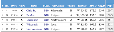
But if you haven't been paying attention to it the offseason, I think you'll be pleasantly surprised, as I've added a bunch of features:
Player Stats—Filters and Leaders since 2010.
One of my projects this summer was to backfill T-Rank, and it now goes back to the 2008-09 season. This includes advanced player stats, though only to 2009-10.
On the Player Finder page, you can look for leaders in various categories in various years, or all time. But the coolest thing (IMO) is the ability to filter out by stat, so that you can look for, say, freshmen in high-major conferences who had a steal rate of at least 4%, and offensive rebounding rate of at least 10%, and a defensive rebounding rate of at least 20%:
It's Ethan. Just Ethan.
Once this season goes live, the 2017 player stats will update in real time.
Game Stats—Filters and Leaders since 2009
Similar to the Player Finder, the Game Finder allows you to look for games matching basically any tempo-free criteria you can imagine. For instance, want to know which B10 teams have scored at least 1.5 points per possession in a Big Ten game since 2009? Here they are:

(At some point I'll probably set this up so you can link to the results of your filtering.)
Team Stats
There's also a specific new page for looking at team leaders in the Four Factors and a few other statistical categories. This, too, is backfilled to 2009. For example, wondering which team had the lowest turnover rate in 2015?
You probably weren't—it was obviously Wisconsin.
These stats can also be filtered by conference and by conference-only stats.
Generate conference championship odds T-Rank WinMatrix in real time.
On the conference pages, you can press the "show odds" button, and T-Rank will simulate that conference's season 50,000 times and show you the results. You can also go the separate Conference Odds page to do the same thing and get a linkable result.
NCAA Tourney Stats
Want to compare tourney results since 2002 by team, by coach, or by conference? T-Rank has you covered.
Generate adjusted efficiency rankings over specific periods or against specified quality of competition.
You already knew about the H-Rank (ranking of every team by their performance over the past 10 games) and Q-Rank (ranking the teams by their performance in "tournament quality tests"). But now using the T-Rank Slice page you can specify your own periods of time to look at—here's last year's results starting at Jan. 1—or by specifying your own cutoff for quality games—here's a look at last year's results against top 25 quality competition. You can even combine them!
T-Ranketology Returns
Friends of the blog know that I tediously overfit T-Ranketology to last year's results. So this year you'll get a full season of tracking your team's tourney chances in real-time. Or you can even tweak the inputs and create your own T-Ranketology!
T-Rank Time Machine
This is actually pretty fun. The T-Rank Time Machine lets you go back and look at T-Rank on a specific day during the past two seasons.
For example, here's Wisconsin on Jan. 12 of last season, when things were looking bleak. If you click through to the conference page, it will even let you run the conference odds as of that day. Notably, T-Rank gave Wisconsin less than a .1% chance of continuing their top-4 steak at that moment. Do you believe in miracles?
So there you go, lots of fun stuff to play around with duing the 2016-17 College Basketball season!
Sunday, October 2, 2016
How much do unbalanced conference schedules matter? Not much.
One of the many downsides of the trend towards mega-conferences is the death of the round-robin conference schedule in basketball. The resulting unbalanced schedules raise the distinct possibility that regular season conference championships will be decided by quirks of scheduling fate rather than talent and coaching tantrums directed at referees as God intended.
The Investigation
But how much difference do unbalanced schedules actually make? To find out, I looked at every season since 2008-09 and used T-Rank to calculate each team's:
1) Expected wins against the conference schedule it actually played;
2) Expected win percentage against a true round robin, and used this to calculate expected wins based on actual number of conference games;
3) Expected chance of winning a share of the title against actual schedule;
4) Expected chance of winning a share of the title against round-robin schedule.
The differences between 1 & 2, and 3 & 4 show the effect of an unbalanced schedule, though in slightly different ways. So I looked at both.
First, the conclusion
Overall, the data is pretty clear that unbalanced schedules are rarely extreme enough to be decisive. By far the dominant force in college basketball is variance, and that's why we love it. All the data is available here.
An Extreme Example: Wisconsin 2016
Let's look at the results for Wisconsin last year as an example.
Expected wins against actual schedule: 10
Expected wins against balanced schedule: 10.8
Chance of winning title against actual schedule: 1.8%
Chance of winning title against balanced schedule: 4%
Obviously, the Badgers got a bad draw last year. Indeed, the -.8 wins is the second most difficult schedule in the entire database. But it's hard to say that even this extreme schedule had much of an effect on anything. The Badgers finished a full 3 games behind Indiana. Even accounting for Indiana's favorable schedule (+.34 expected wins) the Badgers still finished 1.86 adjusted games back:
| Team | Wins | EW Diff | Adj. Wins | Actual EW | Blnced EW | Actual Ch% | Blnced Ch% | Ch% Diff | Adj GB |
| Indiana | 15 | 0.34 | 14.66 | 13.4 | 13 | 29 | 22.4 | 6.6 | 0 |
| Wisconsin | 12 | -0.8 | 12.8 | 10 | 10.8 | 1.8 | 4 | -2.2 | 1.86 |
| Michigan St. | 13 | 0.22 | 12.78 | 14.5 | 14.3 | 61.9 | 56.6 | 5.3 | 1.88 |
| Iowa | 12 | -0.59 | 12.59 | 11.3 | 11.9 | 6.3 | 10.8 | -4.5 | 2.07 |
| Maryland | 12 | -0.37 | 12.37 | 11.5 | 11.9 | 6.8 | 11.8 | -5 | 2.29 |
| Purdue | 12 | -0.2 | 12.2 | 13 | 13.2 | 23.3 | 25.7 | -2.4 | 2.46 |
| Ohio St. | 11 | 0.23 | 10.77 | 8.3 | 8.1 | 0.1 | 0.1 | 0 | 3.89 |
Perhaps more importantly, the Badgers were an extreme long-shot to win the title under a balanced schedule (just 4%) and while the unbalanced schedule cut those long odds by more than half, it's still hard to complain too much about that.
The few examples where it made a difference
Now for the fun stuff: Looking for examples where an unbalanced schedule actually made a difference. First, I looked for teams that didn't win the title and finished less than .5 "adjusted games back." Here they are:
| Team | Year | Conf | Wins | EW Diff | Adj. Wins | Actual EW | Blnced EW | Adj GB |
| Coastal Carolina | 2014 | BSth | 11 | -0.22 | 11.22 | 10 | 10.3 | 0.43 |
| VCU | 2012 | CAA | 15 | 0 | 15 | 14.3 | 14.3 | 0.47 |
| Dayton | 2009 | A10 | 11 | -0.46 | 11.46 | 9.7 | 10.2 | 0.48 |
So just three teams over 7 seasons finished less than .5 adjusted games back, and even these three barely cleared the .5 threshold.
VCU is an interesting one because their schedule actually did not disadvantage them compared to a balanced one. The problem was that that the Colonial champs that year, Drexel, had a very favorable schedule, worth +.53 wins. Most importantly, Drexel only had to play VCU once, and that game was at Drexel. This is when an unbalanced schedule can be really unfortunate: when there is a clear top two that play only once, the team that gets the home game has a big advantage.
The other way I looked at this was to calculate likelihood of winning a championship. I think this is less good than looking at the "adjusted wins" because it's entirely hypothetical. For example, Wisconsin vastly outperformed expectations in conference play last year -- winning 12 games when T-Rank would have expected a team of their quality to win only 10 on overage. As it happened, Indiana also won two more games than expected. But if they'd won 13, as expected, it would have been fair to say that their easier schedule and Wisconsin's harder schedule combined to rob UW of a championship. But if you just look at the simulated difference in Championship expectations (4% vs. 1.8%) for Wisconsin, that doesn't show up.
That said, here are the five teams whose championship odds were negatively affected by 10% or more:
| Team | Conf | Year | Wins | Actual Ch% | Blnced Ch% | Ch% Diff | GB |
| Mount St. Mary's | NEC | 2010 | 12 | 37.1 | 53.9 | -16.8 | 3 |
| VCU | CAA | 2010 | 11 | 28 | 43.5 | -15.5 | 4 |
| VCU | CAA | 2012 | 15 | 48.6 | 60 | -11.4 | 1 |
| Syracuse | BE | 2013 | 11 | 12.9 | 24.3 | -11.4 | 3 |
| Butler | A10 | 2013 | 11 | 15.1 | 26 | -10.9 | 2 |
VCU's 2012 team shows up again, as does its 2010 team. But the 2010 team illustrates the downside of this purely hypothetical analysis: that team actually finished in a tie for 5th pace, a full four games behind Old Dominion. Similarly, each of the other teams (other than 2012 VCU) finished at least 2 games out of first. So although all these teams definitely got screwed by their schedules, they didn't perform well enough to really feel sorry for them.
Caveats
So the overarching conclusion is that most of the time unbalanced schedules are not that big a deal. But a couple caveats:
1) The conclusion that unbalanced schedules don't really affect conference championships doesn't mean that there aren't other effects. Clearly, a tough schedule can easily cost a team one win, and it's not that unusual that one win is the difference between making the NCAA tournament and sitting at home. Pertinently, the 2010 VCU team noted above has a good claim to losing one win based on a bad schedule. That team ended up losing in OT to Old Dominion the Colonial Tournament Championship game, and didn't make the tourney -- despite being No. 51 in Kenpom. It was the next year that VCU snuck into the tournament, as a First Four participant, despite a significantly worse profile, but rode Almighty Variance to the Final Four.
2) Although most schedules are balanced enough most of the time, this is only true in the end. It's still very important to look at who's played whom at a given point in the season. For example, Indiana got a lot of flack about its Big Ten schedule last year, even though in the end it was just marginally favorable. But the real issue was that their schedule was extremely unbalanced temporally, with a very soft 7-game stretch to start. That was a legitimate thing to point out at the time, even though IU continued to surprise even when things got tougher, and cruised to the title in the end.
3) I haven't looked into this systematically, but the trend does seem pretty clear toward more extreme results recently. This is not a surprise, as the rise of the super-conference is relatively recent, and is still in progress. So although we haven't definitely seen it yet, we likely will see an unbalanced schedule decide a major-conference championship soon enough.
Wednesday, September 14, 2016
Who's gaming the RPI this year?
Among the RPI's well-known flaws is that it can be easily gamed. As Luke Winn explained several years ago:
The results are available the T-Rank bubble-rpi page. About half the schedules produce a bubble-team rank between 40-60, which is what you'd expect since the hypothetical bubble team in question would be around #50 in the T-Rank. So bubble-rpi rank around 50 shows that a team's current schedule is reasonably neutral for RPI purposes.
The team with the "best" schedule for maximizing the RPI of a bubble team is North Carolina's. A bubble team playing North Carolina's announced schedule (notably missing two rounds in Maui, including a possible game against Wisconsin), would be expected to go 17-12 and rank 16th in the RPI. Would that be enough to get into the tournament? Assuming those 17 wins include a number of top 50 conquests, I think so. It compares to what Oregon State did last year: 18-12 on Selection Sunday with an RPI rank of 33 and a number of "good wins" got them a 7-seed (!) despite a Kenpom / T-Rank around 60th.
That said, a schedule like North Carolina's is probably not the most advisable for a true bubble team, because it comes to its high ranking rather honestly: by playing a lot of tough games. Sure, the average bubble team would win 17 games, but a bubble team that got a few bad bounces could easily miss the NIT with that schedule.
The schedule with the best mix of good projected record and good projected RPI rank is probably Rhode Island's. A bubble team playing Rhode Island's schedule would project to 21-8 with an RPI rank of 18 -- pretty much a sure thing for the tournament. Rhode Island will also play either Duke or Penn St. in their preseason tournament, in which case the projected RPI rank changes to 17 or 20, respectively. In any case, a bubble team playing that schedule is looking at very likely at least 19 regular season wins and a top 20 RPI. Well done Rams!
How did they do it? The old-fashioned way: lots of beatable mid-majors, and no worthless sub-250 cupcakes. The only downside of their schedule is that it doesn't provide a lot of opportunity for resume-building top-50 wins, and that's why T-Rank currently projects the Rams among the last 4 teams into the tournament (FWIW).
On the flip side, the schedule with the absolute worst RPI profile belongs to North Carolina Central out of the MEAC. A bubble team playing that schedule would be expected to go 22-3 but rank 128th in the RPI. The big problem for NC Central is the MEAC: it has no good teams, and they're all going to get ground to dust in the non-conference.
But of course no potential bubble team plays a schedule like NC Central's, so let's look instead at the worst RPI schedules among high major teams that might have designs on a tournament berth. In that cohort, there are really just four teams that have unusually unfavorable schedules:

Texas Tech rather famously gamed the RPI last year, but Tubby's successor will have a much less favorable slate this year. Their non-conference schedule includes a pathetic seven games against sub-250 projected teams, plus #232 North Texas. That said, they benefit from playing in the Big 12, which projects to be strong top to bottom, so even if they are a bubble-quality team this year (and T-Rank thinks they'll be slightly better than that) they should pick up enough quality wins in conference play to neutralize the stigma of a low raw RPI rank.
Two teams that could suffer from their unfavorable schedules are Utah and Northwestern. Of Utah's eight D-I scheduled non-conference games, six are of the RPI-killing cupcake variety. Throw in Utah's two games against non-DI teams (which don't count for RPI) and 80% of Utah's scheduled non-conference is garbage. Utah does have two games TBD in the Diamond Head Classic, and if they play Illinois St. and San Diego St. that would lift the bubble-projected RPI to 58th. But they've got probably an equal chance of playing Hawaii and Tulsa, which would change the projection back to 68th. Given that Utah could well be a bubble team this year, this schedule could do them in.
Northwestern is less likely to be a bubble-quality team, but if it is its schedule could be a limiting factor. Northwestern also plays six RPI-killing cupcakes. Even more respectable opponents like DePaul and Wake Forest are probably a negative, because those are major conference doormats likely to end up with a bad record -- but they're also very capable of pulling an upset. So it's taking a risk of a loss without any SOS bump.
Ultimately, this exercise illustrates the most damning thing about the RPI: a hypothetical bubble team could finish anywhere between 16th and 128th, completely dependent on its schedule. In other words, the RPI is primarily a metric that measures schedule quality, not team quality.
Seventy-five percent of the RPI formula is about strength of schedule (SOS), and because the RPI uses the flawed metric of raw winning percentage to assess SOS, it fails to provide a true measure of the quality of opponents. The truest measure available is kenpom.com's NCSOS ranking, which creates a pythagorean winning percentage based on opponents' adjusted efficiency, and even adjusts for home/neutral/road situations, which the SOS portion of RPI does not.So in the RPI, your schedule is essentially your destiny. To show this, I set up a hypothetical bubble team (with a pythag of .8000 on a neutral court) and ran the RPI for that team playing every team's announced 2016-17 schedule. Obviously, this excludes later rounds of holiday tournaments and unannounced games, but these have just minor effects at this point.
The results are available the T-Rank bubble-rpi page. About half the schedules produce a bubble-team rank between 40-60, which is what you'd expect since the hypothetical bubble team in question would be around #50 in the T-Rank. So bubble-rpi rank around 50 shows that a team's current schedule is reasonably neutral for RPI purposes.
The team with the "best" schedule for maximizing the RPI of a bubble team is North Carolina's. A bubble team playing North Carolina's announced schedule (notably missing two rounds in Maui, including a possible game against Wisconsin), would be expected to go 17-12 and rank 16th in the RPI. Would that be enough to get into the tournament? Assuming those 17 wins include a number of top 50 conquests, I think so. It compares to what Oregon State did last year: 18-12 on Selection Sunday with an RPI rank of 33 and a number of "good wins" got them a 7-seed (!) despite a Kenpom / T-Rank around 60th.
That said, a schedule like North Carolina's is probably not the most advisable for a true bubble team, because it comes to its high ranking rather honestly: by playing a lot of tough games. Sure, the average bubble team would win 17 games, but a bubble team that got a few bad bounces could easily miss the NIT with that schedule.
The schedule with the best mix of good projected record and good projected RPI rank is probably Rhode Island's. A bubble team playing Rhode Island's schedule would project to 21-8 with an RPI rank of 18 -- pretty much a sure thing for the tournament. Rhode Island will also play either Duke or Penn St. in their preseason tournament, in which case the projected RPI rank changes to 17 or 20, respectively. In any case, a bubble team playing that schedule is looking at very likely at least 19 regular season wins and a top 20 RPI. Well done Rams!
How did they do it? The old-fashioned way: lots of beatable mid-majors, and no worthless sub-250 cupcakes. The only downside of their schedule is that it doesn't provide a lot of opportunity for resume-building top-50 wins, and that's why T-Rank currently projects the Rams among the last 4 teams into the tournament (FWIW).
On the flip side, the schedule with the absolute worst RPI profile belongs to North Carolina Central out of the MEAC. A bubble team playing that schedule would be expected to go 22-3 but rank 128th in the RPI. The big problem for NC Central is the MEAC: it has no good teams, and they're all going to get ground to dust in the non-conference.
But of course no potential bubble team plays a schedule like NC Central's, so let's look instead at the worst RPI schedules among high major teams that might have designs on a tournament berth. In that cohort, there are really just four teams that have unusually unfavorable schedules:
Texas Tech rather famously gamed the RPI last year, but Tubby's successor will have a much less favorable slate this year. Their non-conference schedule includes a pathetic seven games against sub-250 projected teams, plus #232 North Texas. That said, they benefit from playing in the Big 12, which projects to be strong top to bottom, so even if they are a bubble-quality team this year (and T-Rank thinks they'll be slightly better than that) they should pick up enough quality wins in conference play to neutralize the stigma of a low raw RPI rank.
Two teams that could suffer from their unfavorable schedules are Utah and Northwestern. Of Utah's eight D-I scheduled non-conference games, six are of the RPI-killing cupcake variety. Throw in Utah's two games against non-DI teams (which don't count for RPI) and 80% of Utah's scheduled non-conference is garbage. Utah does have two games TBD in the Diamond Head Classic, and if they play Illinois St. and San Diego St. that would lift the bubble-projected RPI to 58th. But they've got probably an equal chance of playing Hawaii and Tulsa, which would change the projection back to 68th. Given that Utah could well be a bubble team this year, this schedule could do them in.
Northwestern is less likely to be a bubble-quality team, but if it is its schedule could be a limiting factor. Northwestern also plays six RPI-killing cupcakes. Even more respectable opponents like DePaul and Wake Forest are probably a negative, because those are major conference doormats likely to end up with a bad record -- but they're also very capable of pulling an upset. So it's taking a risk of a loss without any SOS bump.
Ultimately, this exercise illustrates the most damning thing about the RPI: a hypothetical bubble team could finish anywhere between 16th and 128th, completely dependent on its schedule. In other words, the RPI is primarily a metric that measures schedule quality, not team quality.
Wednesday, August 24, 2016
What's the deal with T-Rank's projection for Indiana?
One of the notable outliers in the official pre-T-Rank is Indiana. Most experts expect IU to contend with Wisconsin, MSU, and Purdue for the Big Ten title and certainly be a top-25 team. Yet T-Rank puts them 30th or so. What gives?
Here is what T-Rank sees:
Here is what T-Rank sees:
- Borderline top 25 program based on last three years' performance (cf: final ranks of 15, 53, and 63 in Kenpom)
- Losing huge star in Yogi Ferrell (87% of minutes, 25% usage, 125 O-Rating) and another major contributor in Troy Williams.
- As a result, returning just 44% of possession-minutes.
- OK recruiting class (20th by T-Rank standards) but nothing special.
Put that together, and T-Rank spits out a projection for 30th. Not as good as last years B1G champs, but a respectable tournament team that's better than the previous two years.
Here's what I think IU fans and IU optimists see instead:
- An elite blue-blood program that has returned to form as evidenced by winning B1G outright last year.
- Exciting young talent like OG Anunoby—who bears a striking resemblance to recent Hoosier great Victor Oladipo—and Thomas Bryant, sophomore studs ready to step up into the open minutes.
Robert JohnsonTroy Williams looks good on paper, but in games he was a chucker and a bad fit—addition by subtraction.- Five freshman, a quality transfer (Newkirk) and a juco guy, all committing to a coach who's a proven identifier of talent.
Look at it that way, and you can see why there's some excitement surrounding IU this preseason.
A fun thing is that we can use the new "Roll Your Own T-Rank" tool to get a pretty plausible version of the pro-IU argument:
- T-Rank punishes IU heavily for Yogi's departure. That's quantified in the "key player lost" parameter. Set that to zero, and IU instantly jumps 12 spots to 18th.
- If you think IU's poor 2014 and 2015 were anomalies, set the weight of those years to 0, so that the program rating is just based on last year. Now IU is all the way to 11th.
So, you can easily get IU to a top-10ish team even in the T-rank if you base program quality on just last year and don't think the loss of Yogi is especially damaging. That's a reasonable position. But so is the T-Rank default: IU has been inconsistent in recent memory, and losing an all-timer at point guard makes it likely they'll regress more to recent program mean.
Will be fun to watch!
Tuesday, August 16, 2016
Non-conference Strength of Schedule
I've begun adding scheduled non-conference games into the 2017 T-Rank projections (courtesy of Reddit user itsbraile's Mega Schedule and a script I wrote to semi-automatically import that data). So I've also added a "Non-conference SOS" column to the 2017 page.
But this is not your daddy's non-conference SOS, so I thought a word of explanation was in order. The way I calculate non-con SOS is to calculate the record that an "elite" team would be expected to have against a given team's schedule. I do this because for good teams there's not much difference, in terms of expected chance of winning, between playing #351 and playing #251 at home -- and this system treats those games as practically identical for SOS purposes.
The NCSOS column on the T-Rank page is actually the expected losing percentage of an elite team against a given schedule, because that way higher is better.
Right now, Long Beach St. has the toughest non-con SOS (as it often does under Dan Monson). (Alabama St. is currently at 1.000 because I don't have any non-con games for their schedule yet). Of course, this will change as we learn more about the actual quality of the teams during the season, as we find out more about the actual non-con schedules, and as later rounds of holiday tournament schedules get on the schedule. So stay tuned!
But this is not your daddy's non-conference SOS, so I thought a word of explanation was in order. The way I calculate non-con SOS is to calculate the record that an "elite" team would be expected to have against a given team's schedule. I do this because for good teams there's not much difference, in terms of expected chance of winning, between playing #351 and playing #251 at home -- and this system treats those games as practically identical for SOS purposes.
The NCSOS column on the T-Rank page is actually the expected losing percentage of an elite team against a given schedule, because that way higher is better.
Right now, Long Beach St. has the toughest non-con SOS (as it often does under Dan Monson). (Alabama St. is currently at 1.000 because I don't have any non-con games for their schedule yet). Of course, this will change as we learn more about the actual quality of the teams during the season, as we find out more about the actual non-con schedules, and as later rounds of holiday tournament schedules get on the schedule. So stay tuned!
Wednesday, July 20, 2016
T-Rank website note
Over the past few days I've been transitioning the T-Rank website (at barttorvik.com) over to a different server on the backend. Short story: everything should work the same and all the old links (well, most of them) should forward automatically to the new corresponding page. So please let me know if you run into any problems.
Long story:
Previously, I used a nifty service called Site44 which turns a folder in your dropbox into a web server. So I would just create all the team pages, conference pages, date pages, etc., every time I ran the T-Rank program, save all the files to a local folder, and they'd magically appear on the web.
The only real problem with this was that some bad people use the Site44 service for nefarious purposes, apparently. So Site44's server IP address was getting banned by some aggressive firewalls. I finally decided to bite the bullet and and set up my own hosted web server on the Amazon cloud service (EC2).
The only problem with this is that my old way of doing things -- creating hundreds of small html files and uploading them every time I made a change -- was no longer practicable, because getting the files to my server in the cloud would take a half-hour or more every time. Instead, I had to learn a new programming language (php) so that I could set up a few template pages which will dynamically create the actual webpages when called. Now I'll just upload a few data files whenever I make changes, and the server takes care of the rest.
Anyhow, we can now add php to python, javascript, jquery, css, and html on the list of programming I've (sort of) learned in bringing T-Rank to the web. Next on the list is SQL. In theory I could potentially turn this new knowledge into something practical someday!
Long story:
Previously, I used a nifty service called Site44 which turns a folder in your dropbox into a web server. So I would just create all the team pages, conference pages, date pages, etc., every time I ran the T-Rank program, save all the files to a local folder, and they'd magically appear on the web.
The only real problem with this was that some bad people use the Site44 service for nefarious purposes, apparently. So Site44's server IP address was getting banned by some aggressive firewalls. I finally decided to bite the bullet and and set up my own hosted web server on the Amazon cloud service (EC2).
The only problem with this is that my old way of doing things -- creating hundreds of small html files and uploading them every time I made a change -- was no longer practicable, because getting the files to my server in the cloud would take a half-hour or more every time. Instead, I had to learn a new programming language (php) so that I could set up a few template pages which will dynamically create the actual webpages when called. Now I'll just upload a few data files whenever I make changes, and the server takes care of the rest.
Anyhow, we can now add php to python, javascript, jquery, css, and html on the list of programming I've (sort of) learned in bringing T-Rank to the web. Next on the list is SQL. In theory I could potentially turn this new knowledge into something practical someday!
Thursday, March 17, 2016
Retrofitting T-Ranketology
I had fun with my hobby project T-Ranketology this year. The results are over at bracketmatrix.com, and I think they're acceptable -- better than major algorithmic projections like KPI and Team Rankings, but worse than most human bracketologists. This makes sense to me, because the tournament selection is a very human affair, and it's hard for a simple model like T-Ranketology to encompass all the vagaries of that process with any real fidelity. As I put it shortly after the bracket was announced: you can't model Madness.
But I will continue to try. To that end, I ran a bunch of experiments to see if I could retrofit T-Ranketology to produce a more accurate bracket. Here are the inputs to T-Ranketology:
RPI
WAB (wins against bubble)
Elo (my E-Rank, a simple elo rating seeded by T-Rank)
"Resume"
Each team was ranked in each of these categories, then their ranks were added up to get a total score (with lower being better). That was T-Ranketology this year.
The "resume" rating needs a better name, and I've got my branding people looking into it. But it was clear to me that bracketology is impossible if you aren't paying attention to "top 50 wins" and the like. So to come up with the Resume rating I used the following point values:
Top 50 win: 10 points
other top 100 win: 3 points:
sub-100 loss: -3 points
sub-200 loss -6 points
Obviously these point values were assigned rather arbitrarily, though I did some experimentation to get a bracket that passed the eye test.
One other possible addition to the algorithm would be T-Rank itself. It's pretty clear that efficiency rating does come into the selection process, at least at the margins. For example, efficiency rating must have been the determining cause of Vanderbilt's inclusion. But it's also ignored a lot, particularly when it comes to seeding.
Anyhow, I've now done a bunch of experiments -- running thousands and thousands of brackets with different values of inputs for each of the T-Ranketology inputs -- to see what the ideal weight of the factors would be. Here are the results:
Resume x 3.5
RPI x 1.5
T-Rank x. 1.5
Elo x 0.25
WAB x 0.2
With Resume being calculated as follows:
Top 25 wins: 16 points
other top 50 wins: 13 points
other top 100 wins: 5 points
sub 100 losses: -1 point
sub 200 losses: -5 points
The original T-Ranketology got a score of 312 on bracketmatrix, by getting 65 teams right, nailing the seed on 31 and within 1 seed on 24 others.
This version of T-Ranketology gets a score of 351 (which would tie for first place this year), by getting 66 teams right, nailing the seed on 44 teams, and within 1 seed on 21 others. This algorithm gets Tulsa and Vanderbilt into the tournament, but leaves Providence and Wichita State as 2nd and 3d teams out, respectively. (St. Bonaventure is the first team out.) Saint Mary's remains in the field, though as a 10-seed instead of an 8-seed. Florida also sneaks into the tournament.
If you want to see the bracket produced by this algorithm, it's here.
Clearly, this version of the algorithm is "over-fit" to this year's results. But I think this exercise does provide some insights. Most obviously, the "resume" rank is extremely important. This is how you get Tulsa into the tournament. You have to really value those wins against "top 25" and "top 50" teams. Bad losses don't matter too much, at least not much more than they already matter for the other ranks. The elo and WAB ratings add a little, but not much, to the analysis.
So, this is the algorithm I'll go with next year. The committee will probably do something entirely different and prove, once again, that you can't model Madness.
But I will continue to try. To that end, I ran a bunch of experiments to see if I could retrofit T-Ranketology to produce a more accurate bracket. Here are the inputs to T-Ranketology:
RPI
WAB (wins against bubble)
Elo (my E-Rank, a simple elo rating seeded by T-Rank)
"Resume"
Each team was ranked in each of these categories, then their ranks were added up to get a total score (with lower being better). That was T-Ranketology this year.
The "resume" rating needs a better name, and I've got my branding people looking into it. But it was clear to me that bracketology is impossible if you aren't paying attention to "top 50 wins" and the like. So to come up with the Resume rating I used the following point values:
Top 50 win: 10 points
other top 100 win: 3 points:
sub-100 loss: -3 points
sub-200 loss -6 points
Obviously these point values were assigned rather arbitrarily, though I did some experimentation to get a bracket that passed the eye test.
One other possible addition to the algorithm would be T-Rank itself. It's pretty clear that efficiency rating does come into the selection process, at least at the margins. For example, efficiency rating must have been the determining cause of Vanderbilt's inclusion. But it's also ignored a lot, particularly when it comes to seeding.
Anyhow, I've now done a bunch of experiments -- running thousands and thousands of brackets with different values of inputs for each of the T-Ranketology inputs -- to see what the ideal weight of the factors would be. Here are the results:
Resume x 3.5
RPI x 1.5
T-Rank x. 1.5
Elo x 0.25
WAB x 0.2
With Resume being calculated as follows:
Top 25 wins: 16 points
other top 50 wins: 13 points
other top 100 wins: 5 points
sub 100 losses: -1 point
sub 200 losses: -5 points
The original T-Ranketology got a score of 312 on bracketmatrix, by getting 65 teams right, nailing the seed on 31 and within 1 seed on 24 others.
This version of T-Ranketology gets a score of 351 (which would tie for first place this year), by getting 66 teams right, nailing the seed on 44 teams, and within 1 seed on 21 others. This algorithm gets Tulsa and Vanderbilt into the tournament, but leaves Providence and Wichita State as 2nd and 3d teams out, respectively. (St. Bonaventure is the first team out.) Saint Mary's remains in the field, though as a 10-seed instead of an 8-seed. Florida also sneaks into the tournament.
If you want to see the bracket produced by this algorithm, it's here.
Clearly, this version of the algorithm is "over-fit" to this year's results. But I think this exercise does provide some insights. Most obviously, the "resume" rank is extremely important. This is how you get Tulsa into the tournament. You have to really value those wins against "top 25" and "top 50" teams. Bad losses don't matter too much, at least not much more than they already matter for the other ranks. The elo and WAB ratings add a little, but not much, to the analysis.
So, this is the algorithm I'll go with next year. The committee will probably do something entirely different and prove, once again, that you can't model Madness.
Tuesday, March 15, 2016
Thoughts on the bracket, part 2: The Snubs
The T-Ranketology algorithm had three teams in the tournament that the selection committee found underserving: St. Bonaventure, Saint Mary's, and South Carolina.
It's pretty obvious what they have in common: they all start with the letter "S". Frankly, anti-S discrimination is as good a theory of why the committee does what it does any other. But let's dig a little deeper into their resumes, and that of the other cause célèbre, Monmouth.
Monmouth
T-Ranketology was not surprised by Monmouth's exclusion, as they were the 12th team out according to the algorithm. This is because they got killed in the "resume" column because of their three bad losses to sub-200 teams.
Monmouth is a tough case because they had the four great wins in the non-conference, against UCLA, USC, Notre Dame, and Georgetown -- all away from home. Since high-major teams have no incentive to play true mids or low-majors on the road, the only path for a team like Monmouth to an at-large bid is go giant slaying on the road, and that's exactly what they did.
Unfortunately, the UCLA and Georgetown wins ended up not looking so great in the committee's eyes, because Georgetown was a sub-100 RPI team and UCLA was 99th. (Indeed, if they'd lost to Georgetown that would counted as a "bad loss"!) This is true even though those were both true road games, which makes them impressive wins by any measure, except any measure the committee pays attention to.
In the end, it was the three sub-200 losses that killed them. I'm pretty sure no team has ever gotten an at-large bid with three losses in that category. This is somewhat unfair to Monmouth, of course, because most at-large contenders do not play very many sub-200 teams on the road. As a result, we don't have an intuitive feel for how often at-large contenders should really lose these games. Monmouth played 11, and they went 8-3. That's not good, but how bad is it?
Easy answer: too bad. I think Monmouth is in the tournament if they go 9-2 in those games. But it was three strikes you're out.
South Carolina
South Carolina was the last team in according to T-Ranketology, and no one is weeping over their omission from the field. They played a crappy schedule, which got them out to a 14-0 start. They were even 20-3, but went just 3-6 in their last nine games. Although their schedule was weak, they actually performed admirably against it, compiling +2.0 WAB, which means they won two more games than you'd expect an average bubble team to win. But (as we'll see) the committee comes down hard on teams that didn't "challenge" themselves during the non-conference, and South Carolina's OOC SOS was 271st according to the RPI.
Since South Carolina is a major conference team that has no excuse for playing such a weak schedule, and they were right on the bubble by all metrics, no one cares about saying sayonara to South Carolina. Hmm, maybe I should write a song called "Sayonara, South Carolina."
Saint Mary's
In my opinion, Saint Mary's was the real snub this year. T-Ranketology had them into the field easily as an 8-seed, and they were in a majority of final brackets at bracketmatrix.com. They had a weak nonconference schedule, but Seth Burn has already detailed how well they performed against the schedule they played, in terms of Wins Against Bubble. They also did well in other metrics traditionally associated with good tourney resumes, such as elo.
Ultimately, they were done in by their lack of "good wins." Their record against the top 100 was great -- 6-3, but the committee cares most about number of wins, not winning percentage. And in the all important "wins against top 50" they had just two. And both those were against Gonzaga, which only squeaked into the top 50 after they beat Saint Mary's in the WCC championship game.
This is a case, I think, where the committee was forced to come face-to-face with the absurdity of its own metrics. Heading into the game against Gonzaga, Saint Mary's had a blank resume, highlighted by zero top-50 wins. They lost that game, convincingly. But now, because of that loss, they had an infinitely better resume, with two top-50 wins. How could a loss possibly improve their resume so much?!
That's a little thing called cognitive dissonance, Jack.
The committee did what anyone does when experiencing cognitive dissonance: it moved on as quickly as possible. Buh-bye, Saint Mary's.
St. Bonaventure
The Bonnies were the last of the S-nubs, and the most surprising, as they were in most every final bracket. But upon examination, their big calling card was a high RPI. The rest of their resume metrics were bubblicious, or worse: 49th in elo, 50th in "resume" (good wins minus bad losses), and 69th in WAB. I shed no tears for St. Bonaventure. Indeed, their exclusion is another sign that raw RPI is (appropriately) not much of an independent factor in the deliberations.
It's pretty obvious what they have in common: they all start with the letter "S". Frankly, anti-S discrimination is as good a theory of why the committee does what it does any other. But let's dig a little deeper into their resumes, and that of the other cause célèbre, Monmouth.
Monmouth
T-Ranketology was not surprised by Monmouth's exclusion, as they were the 12th team out according to the algorithm. This is because they got killed in the "resume" column because of their three bad losses to sub-200 teams.
Monmouth is a tough case because they had the four great wins in the non-conference, against UCLA, USC, Notre Dame, and Georgetown -- all away from home. Since high-major teams have no incentive to play true mids or low-majors on the road, the only path for a team like Monmouth to an at-large bid is go giant slaying on the road, and that's exactly what they did.
Unfortunately, the UCLA and Georgetown wins ended up not looking so great in the committee's eyes, because Georgetown was a sub-100 RPI team and UCLA was 99th. (Indeed, if they'd lost to Georgetown that would counted as a "bad loss"!) This is true even though those were both true road games, which makes them impressive wins by any measure, except any measure the committee pays attention to.
In the end, it was the three sub-200 losses that killed them. I'm pretty sure no team has ever gotten an at-large bid with three losses in that category. This is somewhat unfair to Monmouth, of course, because most at-large contenders do not play very many sub-200 teams on the road. As a result, we don't have an intuitive feel for how often at-large contenders should really lose these games. Monmouth played 11, and they went 8-3. That's not good, but how bad is it?
Easy answer: too bad. I think Monmouth is in the tournament if they go 9-2 in those games. But it was three strikes you're out.
South Carolina
South Carolina was the last team in according to T-Ranketology, and no one is weeping over their omission from the field. They played a crappy schedule, which got them out to a 14-0 start. They were even 20-3, but went just 3-6 in their last nine games. Although their schedule was weak, they actually performed admirably against it, compiling +2.0 WAB, which means they won two more games than you'd expect an average bubble team to win. But (as we'll see) the committee comes down hard on teams that didn't "challenge" themselves during the non-conference, and South Carolina's OOC SOS was 271st according to the RPI.
Since South Carolina is a major conference team that has no excuse for playing such a weak schedule, and they were right on the bubble by all metrics, no one cares about saying sayonara to South Carolina. Hmm, maybe I should write a song called "Sayonara, South Carolina."
Saint Mary's
In my opinion, Saint Mary's was the real snub this year. T-Ranketology had them into the field easily as an 8-seed, and they were in a majority of final brackets at bracketmatrix.com. They had a weak nonconference schedule, but Seth Burn has already detailed how well they performed against the schedule they played, in terms of Wins Against Bubble. They also did well in other metrics traditionally associated with good tourney resumes, such as elo.
Ultimately, they were done in by their lack of "good wins." Their record against the top 100 was great -- 6-3, but the committee cares most about number of wins, not winning percentage. And in the all important "wins against top 50" they had just two. And both those were against Gonzaga, which only squeaked into the top 50 after they beat Saint Mary's in the WCC championship game.
This is a case, I think, where the committee was forced to come face-to-face with the absurdity of its own metrics. Heading into the game against Gonzaga, Saint Mary's had a blank resume, highlighted by zero top-50 wins. They lost that game, convincingly. But now, because of that loss, they had an infinitely better resume, with two top-50 wins. How could a loss possibly improve their resume so much?!
That's a little thing called cognitive dissonance, Jack.
The committee did what anyone does when experiencing cognitive dissonance: it moved on as quickly as possible. Buh-bye, Saint Mary's.
St. Bonaventure
The Bonnies were the last of the S-nubs, and the most surprising, as they were in most every final bracket. But upon examination, their big calling card was a high RPI. The rest of their resume metrics were bubblicious, or worse: 49th in elo, 50th in "resume" (good wins minus bad losses), and 69th in WAB. I shed no tears for St. Bonaventure. Indeed, their exclusion is another sign that raw RPI is (appropriately) not much of an independent factor in the deliberations.
Monday, March 14, 2016
Thoughts on the bracket selection, part 1
I followed the "bracketology" debate more closely than usual this year, for two reasons: (1) until recently, the Badgers were a bubble team (at best), and (2) I used the power of T-Rank to produce an objective bracket prediction (T-Ranketology).
I was satisfied with T-Ranketology's results. It missed three at-larges: Syracuse, Vanderbilt, and Tulsa (instead of Saint Mary's, St. Bonventure, and South Carolina). This was about average for the brackets over at bracketmatrix.com, and if you look at the final "consensus" bracket, T-Ranketology would have had 67 of 68 (with only South Carolina not being a consensus tourney team). Seeding predictions were pretty good, too. All in all, not bad for an algorithm.
There's a lot of hootin' and hollerin' about the committee's selections, and I agree with much of it. But I wanted to take a look at the six teams T-Ranketology was wrong on, plus one other, to see maybe what the committee was thinking and if the algorithm could be improved to reflect that thinking or lack thereof.
Syracuse
Syracuse's overall resume was not great, but the one big trump card they had was a road win at Duke, which is worth like a million resume points. Add a couple other decent (early) wins, and they're left ranked No. 32 in T-Ranketology's "resume" ranking, which is an attempt to simulate the committee's fixation with "top 50" wins, etc. They were also 50th in T-Rank's "wins against bubble" rating, so right on the bubble there. But they were very poor in basic RPI, and had tanked coming down the stretch, leading to a bad elo ranking (which usually pretty well approximates current "sentiments" about how good a team is). All in all, this left Syracuse the sixth team out in T-Ranketology.
But I'm not going to worry about fiddling with T-Ranketology to get Syracuse into the field, because they were clearly a special case.
Vanderbilt
Vanderbilt was the eighth team out in the final T-Ranketology, mainly because it was not in the top 50 of any of the four resume-based metrics the algorithm considered. On the other hand, unlike Syracuse, it was not terrible in any of those metrics, finishing top-70 in all of them.
Clearly Vanderbilt got in because of its efficiency rating. Vandy finished the season ranked 27th in the Kenpom ratings, and top-30 teams always get in nowadays. I think this is why they're slotted in the play-in round against another Kenpom darling, Wichita St.: the committee put two good teams with bad resumes into the ring against each other and said, "If you're so good, prove it."
When I first started T-Ranketology it was loosely modeled after the Easy Bubble Solver, which just averages RPI and Kenpom ranking. Of course, I used T-Rank instead of Kenpom rating, but it was pretty much the same idea. Eventually I took out the efficiency rating component because for good or bad I think it just doesn't play a very big role in the selection or even seeding process, at least not systematically. But I think there's good evidence that it comes into play in edge cases, and I think it's pretty clear that's what got Vandy in. I may have to work in some kind of "top 30" efficiency rating bonus to account for this.
(By the way, I think Syracuse was also helped by a decent Kenpom rating, though I don't think it wouldn't have been enough without The Boeheim Excuse.)
Tulsa
Tulsa was the real shocker, what John Gasaway calls the committee's annual "grenade." But it wasn't a huge shocker to T-Ranketology, which had Tulsa just the fifth team out -- ahead of both Syracuse and Vanderbilt! Indeed, before its loss to Memphis in the AAC tourney on Friday, T-Ranketology had Tulsa the last team in the field.
Why? Like Syracuse, Tulsa scored well in the "resume" score that approximates top 50 wins, etc. This is by far the stupidest possible measure you could come up with, but I'm pleased to say that I think I've done a pretty good job of modeling this particular madness. Tulsa's inclusion in the field of 68 shows that I probably need to weigh it even a little more.
But I think there's another lesson for Tulsa's selection. The committee first gets together early in championship week to get ahead start on the process. As a result, by Friday (when Tulsa got stomped by lowly Memphis) the committee has already made some provisional decisions about which teams it thinks are good enough. I'm pretty sure that Tulsa's resume had already been found deserving by Friday. Here's the way the human mind works: once it decides something, that decision sets. It's like a boulder in a divot; you need a big shove to get it moving again. When new information comes in, we don't start at square one and reevaluate the decision with a blank slate. We say: is this new information enough of a big deal to make me go through this whole process of deciding again? Unsurprisingly, the answer is usually no. This fundamental quality of human psychology (call it laziness if you wish) got Tulsa into the tourney.
(This, by the way, is why college-football-playoff-style in-season tourney rankings are a terrible, terrible idea.)
Well, this has gotten tl;dr so I'm going to stop now. I'll try to post later today with my profound insights into the "snubs."
I was satisfied with T-Ranketology's results. It missed three at-larges: Syracuse, Vanderbilt, and Tulsa (instead of Saint Mary's, St. Bonventure, and South Carolina). This was about average for the brackets over at bracketmatrix.com, and if you look at the final "consensus" bracket, T-Ranketology would have had 67 of 68 (with only South Carolina not being a consensus tourney team). Seeding predictions were pretty good, too. All in all, not bad for an algorithm.
There's a lot of hootin' and hollerin' about the committee's selections, and I agree with much of it. But I wanted to take a look at the six teams T-Ranketology was wrong on, plus one other, to see maybe what the committee was thinking and if the algorithm could be improved to reflect that thinking or lack thereof.
Syracuse
Syracuse's overall resume was not great, but the one big trump card they had was a road win at Duke, which is worth like a million resume points. Add a couple other decent (early) wins, and they're left ranked No. 32 in T-Ranketology's "resume" ranking, which is an attempt to simulate the committee's fixation with "top 50" wins, etc. They were also 50th in T-Rank's "wins against bubble" rating, so right on the bubble there. But they were very poor in basic RPI, and had tanked coming down the stretch, leading to a bad elo ranking (which usually pretty well approximates current "sentiments" about how good a team is). All in all, this left Syracuse the sixth team out in T-Ranketology.
But I'm not going to worry about fiddling with T-Ranketology to get Syracuse into the field, because they were clearly a special case.
The committee chairman had been saying for weeks that Syracuse was going to get special consideration because Syracuse played like shit when Jim Boeheim was serving his 9-game suspension in the middle of the season. Basketball people can look at that argument and see the absurdity on its face -- Syracuse lost five games without Boeheim, and even if you think he is super-god-coach, they almost certainly lose 4 if not all 5 of those games with him. But the committee is not composed of basketball people, so alas. In any event, the handwriting had been on the wall: barring a monumental collapse (which almost happened) Syracuse was going to be in the tournament. If I had been manually fiddling with the T-Ranketolgy bracket, I'd have put Syracuse in for sure.@bkbtNUmbers It certainly should be. But I interpret committee chairman's remarks re Boeheim as "they're in."— Bart Torvik (@totally_t_bomb) March 9, 2016
Vanderbilt
Vanderbilt was the eighth team out in the final T-Ranketology, mainly because it was not in the top 50 of any of the four resume-based metrics the algorithm considered. On the other hand, unlike Syracuse, it was not terrible in any of those metrics, finishing top-70 in all of them.
Clearly Vanderbilt got in because of its efficiency rating. Vandy finished the season ranked 27th in the Kenpom ratings, and top-30 teams always get in nowadays. I think this is why they're slotted in the play-in round against another Kenpom darling, Wichita St.: the committee put two good teams with bad resumes into the ring against each other and said, "If you're so good, prove it."
When I first started T-Ranketology it was loosely modeled after the Easy Bubble Solver, which just averages RPI and Kenpom ranking. Of course, I used T-Rank instead of Kenpom rating, but it was pretty much the same idea. Eventually I took out the efficiency rating component because for good or bad I think it just doesn't play a very big role in the selection or even seeding process, at least not systematically. But I think there's good evidence that it comes into play in edge cases, and I think it's pretty clear that's what got Vandy in. I may have to work in some kind of "top 30" efficiency rating bonus to account for this.
(By the way, I think Syracuse was also helped by a decent Kenpom rating, though I don't think it wouldn't have been enough without The Boeheim Excuse.)
Tulsa
Tulsa was the real shocker, what John Gasaway calls the committee's annual "grenade." But it wasn't a huge shocker to T-Ranketology, which had Tulsa just the fifth team out -- ahead of both Syracuse and Vanderbilt! Indeed, before its loss to Memphis in the AAC tourney on Friday, T-Ranketology had Tulsa the last team in the field.
Why? Like Syracuse, Tulsa scored well in the "resume" score that approximates top 50 wins, etc. This is by far the stupidest possible measure you could come up with, but I'm pleased to say that I think I've done a pretty good job of modeling this particular madness. Tulsa's inclusion in the field of 68 shows that I probably need to weigh it even a little more.
But I think there's another lesson for Tulsa's selection. The committee first gets together early in championship week to get ahead start on the process. As a result, by Friday (when Tulsa got stomped by lowly Memphis) the committee has already made some provisional decisions about which teams it thinks are good enough. I'm pretty sure that Tulsa's resume had already been found deserving by Friday. Here's the way the human mind works: once it decides something, that decision sets. It's like a boulder in a divot; you need a big shove to get it moving again. When new information comes in, we don't start at square one and reevaluate the decision with a blank slate. We say: is this new information enough of a big deal to make me go through this whole process of deciding again? Unsurprisingly, the answer is usually no. This fundamental quality of human psychology (call it laziness if you wish) got Tulsa into the tourney.
(This, by the way, is why college-football-playoff-style in-season tourney rankings are a terrible, terrible idea.)
Well, this has gotten tl;dr so I'm going to stop now. I'll try to post later today with my profound insights into the "snubs."
Thursday, March 10, 2016
Is Kenpom biased in favor of significantly lower-ranked teams? (Yes.)
***
NOTE: Kenpom changed his rating system significantly for the 2017 season (after I did this study) so the results don't necessarily apply to his current system—indeed, there's reason to think the changes he made alleviate the issues discussed below.
***
One of the big problems in college basketball—particularly with regards to NCAA tourney selection—is giving proper weight to road games. It is difficult to intuitively grasp how much harder it is to win on the road against a lesser team than it is to win at home against a better team.
NOTE: Kenpom changed his rating system significantly for the 2017 season (after I did this study) so the results don't necessarily apply to his current system—indeed, there's reason to think the changes he made alleviate the issues discussed below.
***
One of the big problems in college basketball—particularly with regards to NCAA tourney selection—is giving proper weight to road games. It is difficult to intuitively grasp how much harder it is to win on the road against a lesser team than it is to win at home against a better team.
This question came to a head when Greg Shaheen was asked about Wichita State’s big home win over Utah, and specifically what he thought an equivalent road win would be. He answered somewhat absurdly: “Utah.”
Seth Burn set out to answer the question using Kenpom numbers, and what he found was that Wichita State playing No. 25 ranked Utah at home is equivalent to them playing No. 109 rated New Mexico on the road. What this means is that the Kenpom system gives them the same chance (about 73%) of winning in each game.
This is kind of shocking, and my own investigation confirms that it is a correct statement about the Kenpom system. But that doesn’t mean it is necessarily a true fact about the universe. Because Kenpom could be wrong about these things. Importantly, it could be biased in favor of lower-rated home teams.
Indeed, it has been my anecdotal observation that this in fact the case: Kenpom seems to have a systematic bias in favor of significantly lower rated teams when they play higher rated teams, particularly at home. So I set out to test this hypothesis.
First, let’s look at all games that Kenpom would predict the home team to have a margin of victory of +/- one point (favored by 1 or a 1-point underdog). By definition, these will be games where the home team is lower rated than the road team, because home-court advantage is built in. Here are the results:
Games where projected MOV is +/- 1 (Kenpom)
Total games: 372
Home team avg expected MOV: 0.01
Home team actual MOV: -1.81
Home team expected win %: .500
Home team actual win %: .438
What we see in these 372 games that Kenpom would expect to be pretty much pick ‘ems is that the better team (the road team) actually won 56.2% of the time, and had an average margin of victory of +1.8 expectations.
Now, this could just be a quirk of this season—maybe the home teams are just underperforming in close games. But when I run the same test using the T-Rank algorithm, the bias pretty much disappears:
Games where projected MOV is +/- 1 (T-Rank)
Total games: 345
Home team avg expected MOV: 0.06
Home team actual MOV: -0.21
Home team expected win %: .502
Home team actual win %: ..487
This still shows a slight bias toward the (better) road team, but it is much less, and looks much more like random variance.
Next I wanted to test my impression that Kenpom particularly breaks down when the spread between the teams is larger (e.g., games like the nearly 100-spot spread between Wichita St. and New Mexico St.). So I looked at games where the home team was rated more than 50 spots lower than the road team. Using Kenpom projections, here are the results:
Games where home team is more than 50 spots lower than road team (Kenpom)
Total games: 1227
Home team avg expected MOV: -4.34
Home team actual MOV: -6.65
Home team expected win %: .345
Home team actual win %: .271
In this rather large set of games, the home team now actually performs 2.3 points worse, on average, than Kenpom’s system would project, and wins only 80% as often as projected. Compare this to the same experiment with T-Rank:
Games where home team is more than 50 spots lower than road team (T-Rank)
Total games: 1150
Home team avg expected MOV: -6.05
Home team actual MOV: -6.80
Home team expected win %: .311
Home team actual win %: .272
Again, we still see a slight bias in favor of the home team, but a much lower one than with the Kenpom system.
Overall, Kenpom has a very good record of prediction and projection, so if there is a systematic bias in these mismatches, we would expect it to be counterbalanced by good results between more evenly matched teams. And that is in fact the case:
Games where home team and road teams ranked within 50 spots of each other (Kenpom)
Total games: 1804
Home team avg expected MOV: 4.1
Home team actual MOV: 3.58
Home team expected win %: .645
Home team actual win %: .652
(For the record, T-Rank performs similarly in these games, but not quite as good.)
In this set of games, the Kenpom algorithm is extremely well calibrated. My speculation is that the shift from Kenpom 1.0 to Kenpom 2.0 made the algorithm more accurate in these (more common and more important) games, at the expense of some loss of calibration in more mismatched games. This seems worth it, and you can see why it would improve the overall performance of the system.
But I think it’s important to consider this evidence that Kenpom’s projections are systematically based in favor of significantly lower ranked teams when doing this calculation about home/road equivalencies, because the results using Kenpom are not only unintuitive, but in all likelihood just plain wrong.
For example, using T-Rank the equivalent road game to Utah at home for Wichita State is a hypothetical team between No. 83 Temple and No. 84 Hawaii. Utah is ranked 25th in both systems, so this is a great comparison: Kenpom says the road equivalent is No. 109 New Mexico St., and T-Rank says it’s No. 83 Temple or No. 84 Hawaii. Since T-Rank gets better results in these kinds of games, and its results are more in line with most of our intuitions, I’m sticking with T-Rank.
***As to why these difference between T-Rank and Kenpom exist, I believe it has to do with the different "spread" the systems create, and the different "exponents" we use to calculate the Pythagorean Expectation (Kenpom uses 11.5, T-Rank uses 10.25). The different spread is caused mainly by the fact that Kenpom much more aggressively caps margin of victory and the effect of blowouts in mismatches than T-Rank does. My hypothesis is that by mostly ignoring those mismatched games, his system ends up being less accurate in mismatched games, but the upside is that it may be more accurate in games between teams of similar quality.
Subscribe to:
Posts (Atom)